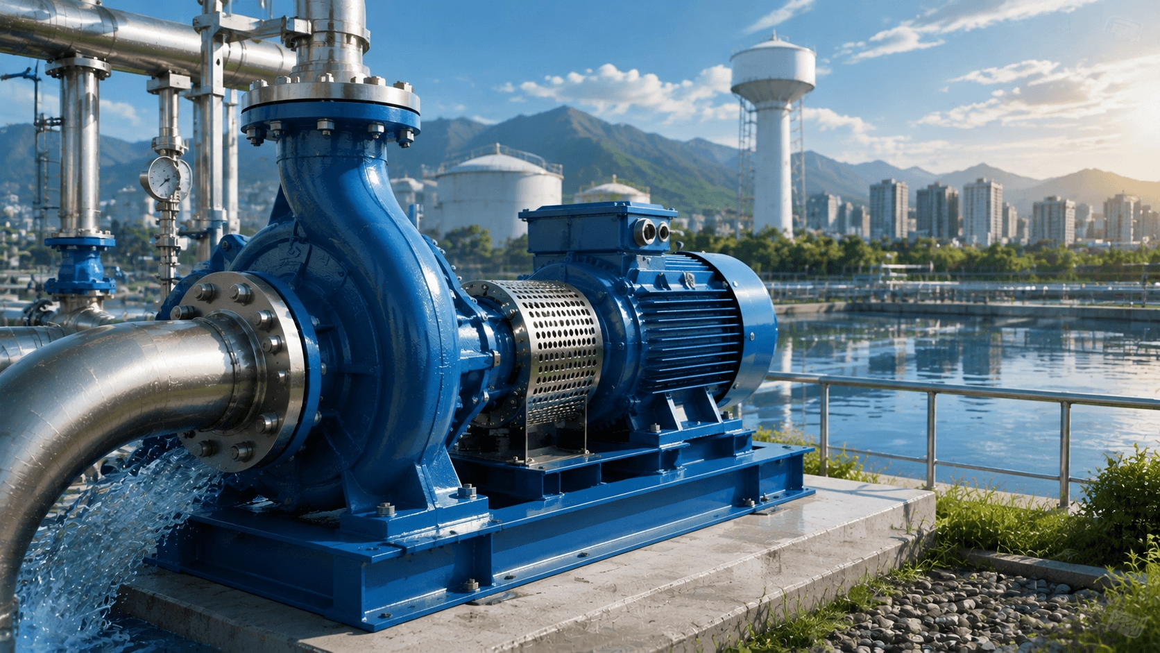
A comprehensive 2026 technical guide to clean water centrifugal pumps covering pump types, specific speed, NPSH engineering, hydraulics, material selection, efficiency optimization, VFD savings, and lifecycle cost analysis.
Table of Contents
- Introduction
- What Is a Clean Water Centrifugal Pump?
- Pump Types and Performance Characteristics
- Specific Speed: The Universal Classification Parameter
- The Affinity Laws and Pump Scaling
- Pump-System Matching and Operating Points
- NPSH Engineering: Preventing Cavitation
- Material Selection for Clean Water Applications
- Motor Efficiency and Energy Optimization
- Lifecycle Cost (LCC) Analysis
- Installation Best Practices
- Maintenance and Reliability
- TITECHO: Precision Motor Engineering
- Pump Selection Workflow Summary
- Frequently Asked Questions
- Conclusion
- Appendix: Quick Reference Formulas
- References
Introduction
Clean water centrifugal pumps are the most widely deployed fluid machinery on Earth. They move drinking water through municipal distribution networks, circulate coolant in power plants, feed boilers in industrial facilities, irrigate millions of hectares of farmland, and maintain pressure in high-rise buildings. Unlike sewage or slurry pumps that must tolerate solids and abrasives, clean water pumps operate in a controlled hydraulic environment where efficiency, reliability, and precision engineering take precedence.
This guide provides a deep technical treatment of clean water centrifugal pump technology—from fundamental hydraulic theory and specific speed classification to material selection, NPSH engineering, energy optimization, and lifecycle cost analysis. Every section includes formulas, performance tables, and engineering guidelines designed for specifying engineers, plant operators, and procurement professionals.
1. What Is a Clean Water Centrifugal Pump?
A clean water centrifugal pump is a rotodynamic machine designed to handle fluids with the following characteristics:
- Low viscosity (typically < 5 cSt, equivalent to water at 20°C)
- Minimal suspended solids (< 0.1% by weight, particle size < 1 mm)
- Neutral pH (typically 6.5–8.5)
- No fibrous or stringy materials
- No gas entrainment (or controlled, < 3% by volume)
These conditions allow the pump to achieve peak hydraulic efficiencies of 80–92%—significantly higher than sewage or slurry pumps—because the impeller can be optimized for pure fluid dynamics rather than solids passage.
1.1 The Energy Equation for Pumping
The fundamental relationship governing pump performance is the Bernoulli equation with pump head addition:
(P1 / rho*g) + (v1^2 / 2g) + z1 + H_pump = (P2 / rho*g) + (v2^2 / 2g) + z2 + H_loss
Where:
- P = Pressure (Pa)
- rho = Fluid density (kg/m³)
- g = Gravitational acceleration (9.81 m/s²)
- v = Flow velocity (m/s)
- z = Elevation (m)
- H_pump = Pump head (m)
- H_loss = Head losses (m)
Rearranging for pump head:
H_pump = ((P2 - P1) / (rho*g)) + ((v2^2 - v1^2) / 2g) + (z2 - z1) + H_loss
2. Pump Types and Performance Characteristics
Clean water applications span an enormous range of flow rates (1 m³/h to 50,000 m³/h) and heads (5 m to 1,000+ m). No single pump type serves all applications. The table below provides a structured comparison.
| Pump Type | Flow Range (m³/h) | Head Range (m) | Max Eff. (%) | Typical Ns Range | Best Application | Motor Position | Cost Index |
|---|---|---|---|---|---|---|---|
| End-Suction Single-Stage | 5–2,000 | 5–150 | 65–88 | 500–2,500 | General water transfer, HVAC | Horizontal, C-frame or close-coupled | 1.0 (baseline) |
| Split-Case Double-Suction | 50–30,000 | 10–250 | 70–92 | 1,000–3,500 | Municipal water supply, irrigation | Horizontal, between bearings | 1.3–1.8 |
| Multi-Stage Ring Section | 5–1,200 | 50–1,200 | 60–82 | 300–1,200 | Boiler feed, high-pressure wash | Horizontal or vertical | 1.5–2.5 |
| Vertical Inline | 5–1,500 | 5–120 | 65–85 | 800–2,500 | Building services, circulation | Vertical inline with pipe | 0.9–1.2 |
| Submersible Clean Water | 10–5,000 | 10–300 | 55–78 | 500–2,000 | Deep well, drainage | Submerged, wet or dry | 1.1–1.4 |
| Self-Priming | 5–500 | 10–80 | 50–70 | 800–2,000 | Sump dewatering, mobile use | Horizontal, above liquid | 1.0–1.3 |
Key Insight: Split-case double-suction pumps achieve the highest efficiency (up to 92%) because the double-entry impeller balances axial thrust and allows higher specific speeds. End-suction pumps offer the best cost-efficiency ratio for general applications.
3. Specific Speed: The Universal Classification Parameter
Specific speed (Ns) is the single most important dimensionless parameter for centrifugal pump classification. It defines the impeller geometry, hydraulic efficiency potential, and operating characteristics.
3.1 Specific Speed Formula
In SI units (with Q in m³/s and H in m):
Ns = (n * sqrt(Q)) / H^0.75
Where:
- n = Rotational speed (rpm)
- Q = Flow rate at BEP (m³/s for single-suction; total flow for double-suction)
- H = Head per stage at BEP (m)
Note: For double-suction pumps, use Q/2 in the formula. For multi-stage pumps, use H divided by the number of stages.
3.2 Specific Speed and Pump Geometry
| Ns Range | Impeller Type | Flow Pattern | Typical Shape | Peak Efficiency | Applications |
|---|---|---|---|---|---|
| 300–800 | Radial (narrow, high blade count) | Radial outward | Deep, narrow vane passages | 65–78% | High-pressure boiler feed, RO |
| 800–1,500 | Francis-type (mixed) | Mixed radial-axial | Moderate width, curved blades | 78–88% | General industrial, municipal water |
| 1,500–2,500 | Mixed flow | Predominantly axial | Wide, swept-back blades | 82–90% | Large water transfer, cooling water |
| 2,500–5,000+ | Axial / Propeller | Axial | Very wide, few blades | 75–85% | Flood control, drainage, irrigation |
Chart Reference Note: H-Q curves for varying specific speed classes demonstrate that low-Ns pumps produce high head at low flow, while high-Ns pumps produce high flow at low head. Peak efficiency typically occurs around Ns ≈ 1,800—the "sweet spot" where impeller geometry optimally balances hydraulic losses.
3.3 Specific Speed Selection Guidelines
To select the appropriate pump type based on flow and head requirements:
- Calculate Ns using the design flow rate and required total head.
- Match Ns to the recommended pump type:
- Ns < 800: Radial flow (end-suction, multi-stage)
- 800–2,500: Mixed flow (split-case, inline)
- Ns > 2,500: Axial flow (propeller)
4. The Affinity Laws and Pump Scaling
The Affinity Laws describe how pump performance changes with speed or impeller diameter. These laws are foundational for variable-speed control and impeller trimming.
4.1 Speed Change
Q2 / Q1 = n2 / n1
H2 / H1 = (n2 / n1)^2
P2 / P1 = (n2 / n1)^3
4.2 Impeller Diameter Change
Q2 / Q1 = D2 / D1
H2 / H1 = (D2 / D1)^2
P2 / P1 = (D2 / D1)^3
4.3 Practical Application: Impeller Trimming vs. Throttling
When a pump is oversized for the system, impeller trimming is far more energy-efficient than throttling.
| Method | Flow Reduction | Head Reduction | Power Reduction | Energy Efficiency |
|---|---|---|---|---|
| Valve Throttling | Reduced | Reduced (wasted) | Slightly reduced | Poor—excess head converted to heat |
| Impeller Trim (D2/D1 = 0.90) | -10% | -19% | -27% | Excellent—matches pump to system |
| VFD Speed Reduction (n2/n1 = 0.90) | -10% | -19% | -27% | Excellent—matches pump to system |
Important Limit: Impeller trimming should not exceed 10–15% of the original diameter for standard pumps, or 20% for high-specific-speed pumps, to avoid excessive efficiency loss and internal recirculation.
5. Pump-System Matching and Operating Points
A pump does not operate in isolation. Its actual performance is determined by the intersection of the pump H-Q curve and the system H-Q curve.
5.1 System Curve Equation
H_system = H_static + k_system * Q^2
Where:
- H_static = Static head (elevation + pressure difference)
- k_system = System resistance coefficient (pipes, fittings, valves)
5.2 Series and Parallel Configurations
- Series Configuration: Used when a single pump cannot achieve the required head. Two identical pumps in series double the head at the same flow. The operating point shifts right along the system curve.
- Parallel Configuration: Used when variable demand requires flow flexibility. Two identical pumps in parallel approximately double the flow at the same head. However, the actual flow gain is typically 50–80% (not 100%) due to the steeper system curve at higher flows.
5.3 Engineering Recommendation for System Matching
Always specify pumps with the ability to trim impellers. A pump selected at 105–110% of design duty and trimmed to match is preferable to an undersized pump that cannot meet future demand. Optimal operation occurs when the pump is precisely matched to the system curve without relying on valve throttling.
6. NPSH Engineering: Preventing Cavitation
Net Positive Suction Head (NPSH) is the critical parameter that determines whether a pump will cavitate. In clean water applications, where vapor pressure is well-defined, NPSH calculations are straightforward but unforgiving.
6.1 NPSH Available Formula
NPSHa = (P_atm / rho*g) - (P_v / rho*g) + H_s - H_f_suction - H_accel
Where:
- P_atm = Atmospheric pressure (varies with altitude)
- P_v = Vapor pressure of water at operating temperature
- H_s = Static suction head (+ if flooded, − if lift)
- H_f_suction = Friction loss in suction piping
- H_accel = Acceleration head (significant in reciprocating suction)
6.2 Atmospheric Pressure vs. Altitude
| Altitude (m ASL) | Atmospheric Pressure (m H₂O) | Correction Factor |
|---|---|---|
| 0 (Sea Level) | 10.33 | 1.000 |
| 500 | 9.71 | 0.940 |
| 1,000 | 9.12 | 0.883 |
| 1,500 | 8.56 | 0.829 |
| 2,000 | 8.02 | 0.776 |
| 2,500 | 7.51 | 0.727 |
| 3,000 | 7.02 | 0.680 |
6.3 Water Vapor Pressure vs. Temperature
| Temperature (°C) | Vapor Pressure (m H₂O) | Vapor Pressure (kPa) |
|---|---|---|
| 10 | 0.12 | 1.23 |
| 20 | 0.24 | 2.34 |
| 30 | 0.43 | 4.24 |
| 40 | 0.75 | 7.38 |
| 50 | 1.23 | 12.35 |
| 60 | 2.03 | 19.92 |
| 70 | 3.12 | 31.16 |
| 80 | 4.83 | 47.39 |
| 90 | 7.18 | 70.14 |
| 100 | 10.33 | 101.33 |
Critical Rule for Hot Water: Always recalculate NPSHa at the maximum expected operating temperature, not merely the design temperature. A pump that is safe at 60°C may cavitate severely at 85°C due to the exponential increase in vapor pressure.
7. Material Selection for Clean Water Applications
Clean water is not always "clean" in the corrosion sense. Temperature, chloride content, dissolved oxygen, and pH all influence material selection.
7.1 Component-Level Material Selection Matrix
| Component | Cold Water (<40°C) | Hot Water (40–90°C) | High Temp (>90°C) | Deionized / Pure Water | Seawater / Brackish |
|---|---|---|---|---|---|
| Impeller | Cast Iron (GG25) | Bronze / SS 304 | SS 316 / Bronze | SS 316 / Plastic | Bronze / Duplex SS |
| Casing / Volute | Cast Iron (GG25) | Cast Iron / SS 304 | SS 316 / Cast Steel | SS 316 | Bronze / Duplex SS |
| Shaft | Carbon Steel (C45) | SS 304 | SS 316 | SS 316 | Duplex SS / Monel |
| Shaft Sleeve | SS 2Cr13 | SS 304 | SS 316 / Stellite | SS 316 / Ceramic | Duplex SS / Titanium |
| Wear Ring | Bronze | Bronze / SS 304 | SS 316 | PTFE / Ceramic | Bronze / Duplex |
| Mechanical Seal | Carbon/Ceramic/NBR | Carbon/SiC/EPDM | SiC/SiC/Viton | SiC/SiC/EPDM | SiC/SiC/Viton |
| Gasket | NBR / EPDM | EPDM / Viton | Viton / Graphite | EPDM / PTFE | Viton / PTFE |
7.2 Material Selection Decision Logic
- Is water temperature > 90°C?
- YES → SS 316 minimum; consider duplex for chloride > 200 ppm.
- NO → Proceed to next step.
- Is chloride > 50 ppm?
- YES → Bronze or SS 304. If chloride > 200 ppm, upgrade to SS 316. If chloride > 1,000 ppm, use Duplex SS (2205) or Super Duplex (2507).
- NO → Proceed to next step.
- Is deionized / pure water?
- YES → SS 316 (avoid cast iron leaching).
- NO → Standard cast iron (GG25) with epoxy coating is acceptable.
8. Motor Efficiency and Energy Optimization
The pump and motor form an integrated energy conversion system. Motor efficiency directly impacts lifecycle cost.
8.1 IEC Motor Efficiency Classes
| Efficiency Class | Min Eff. @ 75% Load (4-pole, 7.5 kW) | Relative Energy Loss | Typical Payback vs IE1 | Regulatory Status | Premium over IE1 |
|---|---|---|---|---|---|
| IE1 (Standard) | 87.0% | 100% (baseline) | — | Phased out (EU) | Baseline |
| IE2 (High Efficiency) | 89.5% | ~82% | 1–2 years | Minimum in EU (2015+) | +10–15% |
| IE3 (Premium Efficiency) | 91.7% | ~65% | 2–4 years | Mandatory in EU (2021+) | +20–35% |
| IE4 (Super Premium) | 93.0% | ~52% | 4–7 years | Voluntary / Incentive | +40–60% |
| IE5 (Ultra Premium) | 94.5% | ~40% | 6–10 years | Emerging standard | +70–100% |
8.2 VFD Energy Savings in Clean Water Systems
Clean water systems often operate at variable load. The energy savings from VFD control follow the cubic affinity law.
| Operating Condition | Flow (% Design) | Speed (% Design) | Power (% Design) | Annual Energy (kWh) | Annual Cost (@ $0.12/kWh) |
|---|---|---|---|---|---|
| Peak Demand | 100% | 100% | 100% | 45,000 | $5,400 |
| Average Demand | 75% | 75% | 42.2% | 18,990 | $2,279 |
| Night / Low Demand | 50% | 50% | 12.5% | 5,625 | $675 |
| Annual Total (VFD) | — | — | — | ~29,000 | ~$3,480 |
| Annual Total (Fixed Speed) | — | — | — | ~45,000 | ~$5,400 |
| Annual Savings | — | — | — | ~16,000 | ~$1,920 |
For a 75 kW pump operating 6,000 hours/year, a VFD retrofit typically pays back in 18–30 months.
9. Lifecycle Cost (LCC) Analysis
The purchase price of a pump is typically less than 15% of its total lifecycle cost. Energy dominates the remaining expenditure.
9.1 LCC Formula
LCC = C_initial + C_energy + C_maintenance + C_downtime + C_decommission
Where:
- C_initial = Purchase + installation + commissioning
- C_energy = Sum of [(P_shaft * t_annual * C_electricity) / (1+r)^t] from t=1 to N
- C_maintenance = Planned + unplanned maintenance over service life
- C_downtime = Lost production / revenue from pump failures
- C_decommission = Removal, disposal, environmental compliance
9.2 LCC Comparison: Standard vs. Premium Pump
| Cost Component | Standard Pump (eta=72%) | Premium Pump (eta=85%) | Savings |
|---|---|---|---|
| Initial Investment | $18,750 | $27,500 | -$8,750 |
| Energy (20 years) | $68,750 | $52,500 | +$16,250 |
| Maintenance (20 years) | $25,000 | $22,500 | +$2,500 |
| Downtime (20 years) | $12,500 | $10,000 | +$2,500 |
| Total LCC (20 years) | $125,000 | $112,500 | +$12,500 |
Conclusion: The premium pump costs 47% more upfront but delivers 10% lower total lifecycle cost over 20 years. The payback period on the efficiency premium is approximately 5–6 years.
10. Installation Best Practices
10.1 Suction Piping Rules
| Parameter | Minimum Recommendation | Critical Limit | Consequence of Violation |
|---|---|---|---|
| Suction pipe diameter | ≥ 1.0× pump suction diameter | < 0.8× | Excessive NPSH loss, cavitation |
| Straight suction length | 5× pipe diameter before pump | < 3× | Flow distortion, uneven impeller loading |
| Eccentric reducer | Flat side up (horizontal pumps) | Concentric reducer | Air pocket formation, vapor locking |
| Suction strainer | Free area ≥ 3× pipe area | < 2× | Excessive pressure drop, starvation |
| Submergence depth | Per manufacturer + 0.3 m margin | < NPSH calculation | Vortex formation, air ingestion |
10.2 Discharge Piping Rules
| Parameter | Recommendation | Notes |
|---|---|---|
| Check valve | Immediately after pump discharge | Prevents backflow and water hammer |
| Isolation valve | After check valve | Allows maintenance without draining system |
| Discharge pipe diameter | ≥ pump discharge diameter | Reduces friction losses |
| Support | Independent of pump flange | Prevents nozzle loading and misalignment |
11. Maintenance and Reliability
11.1 Predictive Maintenance Technologies
| Technology | Monitors | Failure Mode Detected | Implementation Cost | ROI Timeline |
|---|---|---|---|---|
| Vibration Analysis | Bearing condition, imbalance, misalignment | Bearing failure, impeller damage, coupling wear | 2,000–5,000 / point | 6–12 months |
| Temperature Monitoring | Bearing temp, motor winding | Lubrication failure, overload, seal leakage | 500–1,500 / point | 3–6 months |
| Current Signature Analysis | Motor electrical health | Rotor bar cracks, eccentric air gap | 3,000–8,000 / motor | 12–18 months |
| Seal Leak Detection | Mechanical seal condition | Seal failure, environmental release | 200–800 / pump | Immediate |
| Pressure / Flow Monitoring | System performance | Internal wear, impeller trimming, valve degradation | 1,000–3,000 / system | 6–12 months |
11.2 Mean Time Between Failures (MTBF) by Strategy
| Maintenance Strategy | MTBF (hours) | MTBF (months) | Key Practices |
|---|---|---|---|
| Reactive (Breakdown) | ~4,000 | ~5.5 | Fix when failed; highest lifecycle cost |
| Preventive (Time-based) | ~8,000 | ~11.0 | Scheduled overhaul; moderate cost |
| Predictive (Condition-based) | ~12,000 | ~16.4 | Vibration, temperature monitoring |
| Reliability-Centered (RCM) | ~16,000 | ~21.9 | Root-cause analysis; design optimization |
12. TITECHO: Precision Motor Engineering
TITECHO specializes in hollow-shaft motors engineered for direct coupling with high-pressure pump heads—such as the Hawk AR series used in industrial pressure-washing and RO systems. While core expertise lies in hollow-shaft platforms, the engineering principles of motor-pump integration, thermal management, and efficiency optimization apply universally across clean water applications.
12.1 Motor-Pump Integration Philosophy
The motor and pump are not separate purchases—they are a mechanical and thermal system. TITECHO approaches every application with system-level thinking:
- Thermal Management: Class F or H insulation with temperature rise reserves; independent cooling fan for VFD duty; bearing temperature monitoring as a standard option.
- Mechanical Integration: Hollow-shaft design eliminates coupling misalignment; precision-machined shaft extensions for direct pump coupling; custom flange interfaces for split-case and vertical turbine pumps.
- Electrical Performance: 100% copper windings for minimal I²R losses; cold-rolled silicon steel laminations (0.5 mm) for low core losses; IE3 as standard with IE4 and IE5 available; dual-voltage configurations.
12.2 Customization Capabilities
| Feature | Standard | Optional |
|---|---|---|
| Power Range | 0.75 kW – 315 kW | Up to 630 kW on request |
| Voltage / Frequency | 380V/50Hz, 460V/60Hz | 220V–690V, 50/60Hz, dual-voltage |
| Efficiency Class | IE3 (Premium) | IE4, IE5 |
| Protection Rating | IP55 | IP56, IP65, IP66 |
| Cooling | IC411 (fan-cooled) | IC416 (independent fan), IC418 (air-to-air) |
| Thermal Protection | PTC thermistors (3 per phase) | PT100 (bearing + winding), PT1000 |
| Bearings | Standard deep-groove ball | SKF, NSK, FAG; insulated for VFD |
| Shaft Material | C45 carbon steel | SS 304, SS 316, 17-4PH |
| Mounting | IM B3 (foot), IM B5 (flange) | IM B35, IM V1, IM V3, custom |
| Paint | Standard epoxy (RAL 5010) | Marine grade, C5-M, custom colors |
12.3 Application-Specific Solutions
- Boiler Feed Pumps: High-speed motors (2-pole, 2,900–3,600 rpm) matched to multi-stage ring section pumps; thrust bearing arrangements for high axial loads; Class H insulation.
- Municipal Water Supply: 4-pole motors (1,450 rpm) for split-case double-suction pumps; IE3/IE4 efficiency for continuous duty; VFD-ready with independent cooling.
- HVAC Circulation: Compact vertical inline motor designs; low-noise bearing configurations; dual-speed or VFD-compatible for part-load efficiency.
- Irrigation: Weatherproof enclosures (IP56+) for outdoor installation; high-starting-torque designs; robust shaft seals for dusty environments.
13. Pump Selection Workflow Summary
Use this structured process to specify a clean water centrifugal pump:
- Define Hydraulic Requirements: Determine design flow rate (peak demand + 1.1–1.25× safety margin) and total dynamic head (static + friction + minor losses + discharge pressure).
- Calculate Specific Speed: Compute Ns and match to pump type using the guidelines in Section 3.
- Calculate NPSHa: Verify NPSHa >= NPSHr + 1.5 m at all operating conditions, accounting for altitude, temperature, and worst-case suction scenarios.
- Select Pump and Impeller: Choose pump type, verify efficiency at expected operating range (target > 85% of peak eta), and confirm impeller trim range covers the design point.
- Size the Motor: Calculate shaft power and select a motor with a minimum 1.15 service factor. For VFD duty, specify inverter-rated motor with Class F insulation and independent cooling.
- Verify System Integration: Check pipe velocities (suction 0.9–2.5 m/s; discharge 1.5–3.5 m/s), confirm sump/submergence requirements, and specify appropriate valves and instrumentation.
- Lifecycle Cost Validation: Calculate 20-year LCC including energy, maintenance, and downtime. Compare standard vs. premium efficiency options and evaluate VFD payback.
14. Frequently Asked Questions
- What is the difference between a clean water pump and a sewage pump?
- Can a clean water pump handle slightly dirty water?
- How do I know if my pump is cavitating?
- Is VFD control always better than throttling?
- What is the maximum allowable impeller trim?
- Should I specify IE4 or IE5 motors?
(Detailed answers to these questions should be developed based on project-specific parameters and manufacturer data.)
15. Conclusion
Clean water centrifugal pump selection is a disciplined engineering exercise that balances hydraulic performance, energy efficiency, material compatibility, and lifecycle economics. The formulas, charts, and tables in this guide provide the analytical tools for making technically sound decisions—but the final specification must always account for site-specific conditions, regulatory requirements, and operational constraints.
The most successful pump installations result from close collaboration between the pump manufacturer, the motor supplier, the system designer, and the end-user operations team. No catalogue selection can replace the value of application engineering.
For technical consultation on motor selection, hollow-shaft configurations, efficiency upgrades, or custom engineering for your clean water pumping system, contact the TITECHO team.
Appendix: Quick Reference Formulas
| Formula | Application |
|---|---|
| H = ((P2-P1)/(rho*g)) + ((v2^2-v1^2)/2g) + (z2-z1) + H_loss | Bernoulli with pump head |
| P_shaft = (rho * g * Q * H) / (3600 * 1000 * eta_pump) | Shaft power (kW) |
| Ns = (n * sqrt(Q)) / H^0.75 | Specific speed (SI units) |
| NPSHa = ((P_atm - P_v)/(rho*g)) + H_s - H_f | NPSH available |
| Q2/Q1 = n2/n1 ; H2/H1 = (n2/n1)^2 ; P2/P1 = (n2/n1)^3 | Affinity laws (speed) |
| H_system = H_s + k_system * Q^2 | System curve |
| H2/H1 = (D2/D1)^2 | Impeller trimming law |
| Re = (rho * v * D) / mu | Reynolds number |
| H_f = f * (L/D) * (v^2 / 2g) | Darcy-Weisbach friction loss |
| LCC = C_initial + C_energy + C_maint + C_down | Lifecycle cost |
References
- Centrifugal Pump Handbook, Sulzer Pumps Ltd., 4th Edition
- Pump Handbook, Karassik, Messina, Cooper, Heald, 4th Edition
- ISO 9906:2012 — Rotodynamic pumps — Hydraulic performance acceptance tests
- ISO 5199:2002 — Technical specifications for centrifugal pumps — Class II
- ANSI/HI 9.6.1 — Rotodynamic Pumps — Guideline for NPSH Margin
- IEC 60034-30-1 — Rotating electrical machines — Efficiency classes (IE code)
- Hydraulic Institute Engineering Data Book, Hydraulic Institute, 2nd Edition