1. Introduction: Why VFD Pumps Revolutionize Fluid Systems
The centrifugal pump is a slave to its system curve. In a fixed-speed installation, the pump can only operate at the single intersection point between its head-capacity curve and the system resistance curve. When system demand changes—which it always does—the pump responds by throttling, bypassing, or cycling on and off. All three methods waste energy, accelerate wear, and degrade process control.
The Variable Frequency Drive (VFD) pump changes this fundamental constraint. By modulating the electrical frequency supplied to the motor, the VFD shifts the entire pump curve in real time, matching hydraulic output to actual system demand. The result is not incremental improvement—it is a transformation in energy efficiency, equipment longevity, and process precision.
This guide provides the complete engineering framework for VFD pump selection, the affinity laws that govern variable-speed operation, energy savings calculations, and the system design considerations that separate successful installations from costly failures.
2. The Three Affinity Laws: The Mathematics of Variable Speed
The affinity laws are not approximations—they are derived from dimensional analysis of rotating machinery and describe exact relationships for dynamically similar operating conditions. For a given impeller diameter, speed changes produce predictable, mathematically exact changes in flow, head, and power.
Formula 1: The Three Pump Affinity Laws
| Affinity Law | Relationship | Engineering Significance |
|---|---|---|
| Law 1: Flow vs. Speed | Q₁/Q₂ = N₁/N₂ | Flow changes linearly with speed. A 20% speed reduction yields exactly 20% less flow. |
| Law 2: Head vs. Speed | H₁/H₂ = (N₁/N₂)² | Head changes with the square of speed. A 20% speed reduction yields 36% less head (1 − 0.8² = 0.36). |
| Law 3: Power vs. Speed | P₁/P₂ = (N₁/N₂)³ | Power changes with the cube of speed. A 20% speed reduction yields 48.8% less power (1 − 0.8³ = 0.488). |
The Cubic Law is the economic engine of VFD technology. Because power consumption falls with the cube of speed reduction, even modest speed adjustments produce dramatic energy savings. A pump running at 80% speed consumes only 51% of full-speed power. At 70% speed, it consumes only 34%. This is not theory—it is the physical law that makes VFD payback periods routinely fall below 18 months.
Formula 2: Combined Affinity Law for Speed & Impeller Diameter Changes
When both speed and impeller diameter change simultaneously:
Q₁/Q₂ = (N₁/N₂) · (D₁/D₂)
H₁/H₂ = (N₁/N₂)² · (D₁/D₂)²
P₁/P₂ = (N₁/N₂)³ · (D₁/D₂)⁵
Important Limitation: The affinity laws assume geometric similarity and constant efficiency. They are accurate for speed ratios between 0.5 and 1.5. Beyond this range, Reynolds number effects, NPSH limitations, and mechanical resonance can cause significant deviation. Always verify with manufacturer test data for extreme speed changes.
3. VFD Energy Savings: Quantifying the Economic Impact
Formula 3: Annual Energy Savings Calculation
The energy savings from VFD installation depend on the pump's duty profile—the percentage of time spent at each flow rate.
Annual Savings (kWh) = Σ [(P_fixed,i − P_VFD,i) · t_i] / η_motor
Where:
- P_fixed,i = Power at flow rate Q_i with fixed-speed operation (throttling or bypass)
- P_VFD,i = Power at flow rate Q_i with VFD speed control
- t_i = Hours per year at flow rate Q_i
- η_motor = Motor efficiency (typically 0.88–0.95)
For throttled fixed-speed systems:
P_fixed = (Q · H_pump) / (η_p · 3960) · (0.746 / η_motor)
(Where H_pump is the head produced by the pump at flow Q following the pump curve, regardless of system demand.)
For VFD-controlled systems:
P_VFD = (Q · H_system) / (η_p · 3960) · (0.746 / (η_motor · η_VFD))
(Where H_system is the actual head required by the system at flow Q following the system curve, and η_VFD is the drive efficiency, typically 0.95–0.98.)
The difference between H_pump and H_system represents the throttling loss—energy dissipated as heat across control valves. The VFD eliminates this loss entirely.
Formula 4: Simplified VFD Savings Formula
For systems where flow varies according to a known profile, the cubic relationship yields a direct savings estimate:
Energy Savings (%) = 100 × [1 − (f₂/f₁)³]
Where: f₁ = base frequency (typically 50 or 60 Hz) and f₂ = reduced operating frequency.
Worked Example:
A 75 kW irrigation pump operates at full speed (50 Hz) for 2,000 hours/year and at 70% speed (35 Hz) for 4,000 hours/year.
Fixed-Speed Operation (throttled):
- At full flow: 75 kW × 2,000 h = 150,000 kWh
- At reduced flow (throttled to 70%): 75 kW × 4,000 h = 300,000 kWh
- Total: 450,000 kWh
VFD Operation:
- At full flow: 75 kW × 2,000 h = 150,000 kWh
- At 70% speed: 75 kW × (0.7)³ × 4,000 h = 75 × 0.343 × 4,000 = 102,900 kWh
- Total: 252,900 kWh
Annual Savings: 450,000 − 252,900 = 197,100 kWh
- At 0.12/kWh: **23,652/year**
- With VFD installed cost of $25,000: Payback = 12.7 months
4. VFD Pump Performance Analysis
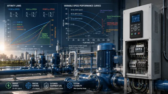
Chart 1: Affinity Laws & Variable Speed Performance Curves
Left Panel — Affinity Law Relationships & Energy Savings:
This chart visualizes the three affinity laws and their engineering consequences:
- Flow Rate (Blue): Linear relationship. At 50% speed, flow is exactly 50%. This is intuitive and predictable.
- Head (Green, dashed): Square relationship. At 50% speed, head drops to 25%. This means the pump cannot maintain high pressure at low speeds—a critical limitation for high-static-head systems.
- Power (Red, dash-dot): Cubic relationship. At 50% speed, power drops to 12.5%. This is the economic foundation of VFD technology. The green shaded area between the power curve and the flow curve represents the energy savings versus throttling.
- Efficiency (Orange, secondary axis): Pump efficiency remains relatively constant across the 60–100% speed range but drops at very low speeds (< 50%) due to increased proportion of mechanical losses relative to hydraulic power.
Key Operating Points:
- 100% speed: 100% flow, 100% head, 100% power
- 80% speed: 80% flow, 64% head, 51% power → 49% energy savings
- 70% speed: 70% flow, 49% head, 34% power → 66% energy savings
- 60% speed: 60% flow, 36% head, 22% power → 78% energy savings
- 50% speed: 50% flow, 25% head, 12.5% power → 87.5% energy savings
Right Panel — Variable Speed Performance Curves & System Matching:
This chart shows how a VFD shifts the entire pump curve to match system demand:
- 50 Hz (Dark Blue): Full-speed curve. Intersects the Peak Demand System at Q = 108 m³/h, H = 32.5 m, with η = 80%.
- 40 Hz (Medium Blue): 80% speed curve. Matches the Normal Demand System at Q = 72 m³/h, H = 18.2 m, with η = 78%. Power is only 51% of rated.
- 30 Hz (Light Blue): 60% speed curve. Matches the Low Demand System at Q = 42 m³/h, H = 9.8 m, with η = 72%. Power is only 22% of rated.
The red vertical line shows throttling loss: If the fixed-speed pump were throttled to meet normal demand, it would produce 32.5 m of head but the system only needs 18.2 m. The difference (14.3 m) is pure energy waste. The VFD eliminates this entirely.
5. VFD vs. Throttling vs. Impeller Trimming: The Control Method Decision
Table 1: Flow Control Method Comparison
| Control Method | Energy Efficiency | Flexibility | Initial Cost | Maintenance | Best Application |
|---|---|---|---|---|---|
| Throttling (Valve) | Poor (wastes head) | Good (real-time) | Low | High (valve wear) | Temporary/seasonal |
| Bypass Recirculation | Very Poor | Good | Low | Moderate | Min. flow requirements |
| On/Off Cycling | Poor (frequent starts) | Poor | Very Low | Very High | Small, intermittent |
| Impeller Trimming | Good (permanent) | None (fixed) | Low (500–2k) | Low | Constant reduced-flow |
| VFD Speed Control | Excellent | Excellent (0-100%) | High (8k–25k) | Low | Variable, continuous |
| Multiple Fixed-Speed | Moderate (step) | Moderate | Moderate | Moderate | Discrete flow steps |
Selection Decision Tree:
- Does flow vary > 30% from design point for > 30% of operating hours?
- Yes → VFD is economically justified.
- No → Consider impeller trimming or fixed-speed with throttling.
- Is demand predictable and constant?
- Yes → Impeller trimming is most cost-effective.
- No → VFD provides necessary flexibility.
- Is the system open-loop (irrigation) or closed-loop (HVAC)?
- Open-loop → VFD savings are harder to predict; verify with duty profile analysis.
- Closed-loop → VFD savings are typically 20–50%.
6. VFD System Design: Engineering Considerations
Table 2: VFD Specification Parameters
| Parameter | Specification | Engineering Impact |
|---|---|---|
| Input Voltage | 380–480V, 3-phase (std) or 690V | Must match motor nameplate; voltage imbalance < 2% |
| Output Freq. Range | 0–60 Hz (std) or 0–400 Hz | Minimum speed typically 30% for self-cooled motors |
| Carrier Frequency | 2–16 kHz (default 4–6 kHz) | Higher = quieter, higher VFD losses; lower = more motor heat |
| Overload Capacity | 150% for 60 seconds (std) | Must exceed pump starting torque requirements |
| Harmonic Dist. (THDi) | < 5% with filter; < 30% without | IEEE 519 compliance; may require line reactors |
| Efficiency | 95–98% at rated load | Account for 2–5% additional losses in savings calcs |
| Enclosure Rating | IP20 (panel) to IP66 (outdoor) | Match installation environment |
| Control Interface | 4–20 mA, 0–10V, Modbus, BACnet | Match to plant control system architecture |
Formula 5: Minimum VFD Speed for Motor Cooling
Standard TEFC (Totally Enclosed Fan Cooled) motors rely on shaft-mounted fans. At low speeds, cooling airflow drops linearly with speed while motor losses remain relatively constant.
N_min = N_rated · [P_loss / (P_loss + P_cooling,base)]
For most TEFC motors:
N_min ≈ 0.30 · N_rated
Below 30% speed, specify:
- Force-ventilated motor with independent cooling fan
- Submersible motor (liquid-cooled, speed-independent)
- VFD with motor derating function that limits torque at low speed
Formula 6: VFD Output Cable Length & dv/dt Effects
VFDs produce PWM (Pulse Width Modulation) waveforms with rapid voltage rise times (dv/dt). Long cables between VFD and motor create voltage reflections that can damage motor insulation.
L_max = [1 / (6 · f_carrier · v_prop)] · [V_dc / (dv/dt)_max]
Where:
- f_carrier = VFD carrier frequency (Hz)
- v_prop = Propagation velocity in cable (~150 m/μs)
- V_dc = DC bus voltage (~1.35 × AC line voltage)
- (dv/dt)_max = Motor insulation withstand rate (typically 500–1500 V/μs)
Practical Limits:
| Motor Insulation Class | Max Cable Length (unfiltered) | Mitigation Required Beyond |
|---|---|---|
| Standard (≤ 600V) | 50 m | Output reactor or dV/dt filter |
| Inverter-duty (≤ 1000V) | 150 m | Sine wave filter |
| Inverter-duty + filter | 300 m | None |
7. NPSH Considerations for VFD Pumps
Formula 7: NPSH Available vs. Speed
NPSH available is independent of pump speed—it depends only on system conditions:
NPSH_a = (P_atm − P_vapor) / (ρ · g) + H_static − H_f,suction
However, NPSH required increases with speed squared:
NPSH_r,1 / NPSH_r,2 = (N₁ / N₂)²
Critical VFD Design Rule: At maximum speed, verify:
NPSH_a ≥ NPSH_r,max + 1.5 m
Table 3: NPSH Safety Margins for VFD Operation
| Application | NPSH Margin at 100% Speed | NPSH Margin at 120% Speed | Action if Insufficient |
|---|---|---|---|
| Clean water, cold (< 30°C) | ≥ 1.0 m | ≥ 2.5 m | Reduce max speed; increase suction pressure |
| Hot water (> 60°C) | ≥ 2.0 m | ≥ 4.0 m | Install booster pump; reduce fluid temperature |
| High suction lift | ≥ 1.5 m | ≥ 3.0 m | Lower pump elevation; increase suction pipe size |
| Submersible (flooded) | ≥ 0.5 m | ≥ 1.5 m | Typically not a concern; verify at max speed |
8. Harmonics, Power Quality & Electrical Design
VFDs draw non-sinusoidal current from the power supply, creating harmonic distortion. This affects not only the VFD itself but all equipment on the same electrical bus.
Formula 8: Total Harmonic Distortion (THD)
THD_i = [√(Σ I_h²) / I₁] × 100%
IEEE 519 Limits:
| Voltage Level | Max THD_v | Max THD_i (I_sc/I_L < 20) |
|---|---|---|
| ≤ 69 kV | 5% | 5% |
| 69–161 kV | 3% | 2.5% |
| > 161 kV | 1.5% | 1.5% |
Harmonic Mitigation Options:
| Method | THD_i Reduction | Cost | Best For |
|---|---|---|---|
| AC Line Reactor (3%) | 30–40% | Low | Small systems, < 50 kW |
| DC Link Choke | 30–40% | Low | New VFD installations |
| 12-Pulse VFD | 70–80% | Moderate | Large systems, > 100 kW |
| Active Front End (AFE) | > 95% | High | Critical, IEEE 519 compliance |
| Passive Harmonic Filter | 80–90% | Moderate | Retrofit applications |
Motor Derating for VFD Service:
Standard motors should be derated 5–15% for VFD service unless specifically rated "inverter-duty." Inverter-duty motors feature enhanced insulation (Class H with Class F temperature rise), separate cooling fans, and bearing insulation to prevent shaft currents.
9. Control Strategies for VFD Pumps
Table 4: VFD Control Modes & Applications
| Control Mode | Sensor Input | Setpoint | Best Application | Response Speed |
|---|---|---|---|---|
| Constant Pressure | Pressure transducer | Fixed pressure (e.g., 4.0 bar) | Water supply, boosters | Fast (< 2 s) |
| Constant Flow | Flow meter | Fixed flow rate (e.g., 50 m³/h) | Process dosing, cooling | Moderate (5–10 s) |
| Constant Level | Level transmitter | Fixed tank level (e.g., 3.5 m) | Sump drainage, reservoirs | Slow (10–30 s) |
| Proportional Press. | Pressure + flow | Pressure varies with flow (PID) | HVAC, variable networks | Fast (< 2 s) |
| Multi-Pump Cascade | Pressure/level | Staged pump activation | Large systems, wide demand | Staged |
PID Tuning for VFD Pump Control
The VFD PID controller adjusts motor speed to maintain the process variable at setpoint:
Output = K_p · e(t) + K_i · ∫e(t)dt + K_d · de(t)/dt
Where: e(t) = setpoint − measured value.
Recommended PID Settings for Pump Applications:
| Application | K_p | K_i | K_d | Integral Time (T_i) |
|---|---|---|---|---|
| Pressure control (water) | 1.0–2.0 | 0.1–0.3 | 0.0–0.1 | 10–30 s |
| Flow control (process) | 0.5–1.5 | 0.05–0.2 | 0.0–0.05 | 20–60 s |
| Level control (drainage) | 0.3–0.8 | 0.02–0.1 | 0.0–0.02 | 60–180 s |
Note: Anti-Windup is essential for pump applications. If the VFD output saturates at minimum or maximum speed, the integral term must be clamped to prevent overshoot when demand returns.
10. Multi-Pump VFD Systems: Cascade Control
For systems with wide demand variation, a single oversized VFD pump is inefficient at low flows. The solution is cascade control with multiple pumps.
Table 5: Multi-Pump Cascade Configuration
| Configuration | Pump Count | VFD Count | Energy Efficiency | Capital Cost | Best For |
|---|---|---|---|---|---|
| Lead VFD + Fixed Lag | 2–4 | 1 | Good | Low | Moderate demand variation |
| Lead VFD + Lag VFD | 2–4 | 2 | Very Good | Moderate | High demand variation |
| All VFD (1 per pump) | 2–4 | 2–4 | Excellent | High | Critical, precise control |
| VFD + DOL Staging | 3–6 | 1 | Moderate | Lowest | Large, budget-constrained |
Lead VFD + Fixed Lag Logic:
- VFD pump starts at minimum speed.
- As demand increases, VFD speeds up to 100%.
- At 100% VFD + demand still rising → start fixed-speed lag pump, VFD resets to ~60%.
- Repeat for additional pumps. Reverse sequence on demand reduction.
Lead VFD + Lag VFD Logic:
- Lead VFD pump modulates 0–100%.
- At ~90% lead VFD → start lag VFD at minimum speed.
- Both VFDs share load equally (same speed).
- Continue staging additional VFD pumps as needed.
Energy Advantage: Multiple smaller VFD pumps operating near BEP are typically 10–20% more efficient than one oversized pump throttled to partial load.
11. Lifecycle Cost Analysis: VFD vs. Fixed-Speed
Table 6: 15-Year Lifecycle Cost Comparison (75 kW Pump, 6,000 hrs/year)
| Cost Component | Fixed-Speed + Throttling | VFD Speed Control |
|---|---|---|
| Initial Equipment | $18,000 (pump + motor + valve) | $35,000 (pump + motor + VFD + filter) |
| Installation | $5,000 | $8,000 |
| Annual Energy (Year 1) | $48,600 | $32,400 |
| 15-Year Energy (3%/yr) | $907,000 | $604,700 |
| Maintenance & Parts | $85,000 (valves, motor overhauls) | $45,000 (VFD capacitor replacement) |
| Downtime / Lost Prod. | $35,000 | $12,000 |
| Residual Value | -$3,000 | -$5,000 |
| TOTAL LCC | $1,057,000 | $727,700 |
- Net Present Value Savings: $329,300 over 15 years
- Simple Payback: 2.1 years
- Internal Rate of Return: 42%
12. Troubleshooting VFD Pump Systems
| Symptom | Diagnostic | Root Cause | Corrective Action |
|---|---|---|---|
| Motor overheating | Check current waveform; measure winding temp | Insufficient cooling at low speed; harmonic heating | Install forced ventilation; verify carrier frequency; check motor rating |
| Excessive noise/vibration | Spectrum analysis; check mounting | Bearing currents (shaft voltage); mechanical resonance | Install shaft grounding ring; check for critical speed excitation |
| VFD overcurrent trip | Review fault history; check load profile | Pump clogging; mechanical seizure; acceleration too fast | Inspect pump; clear blockage; increase ramp time |
| Pressure oscillation | Monitor PID output; check sensor signal | PID tuning too aggressive; sensor noise; valve hunting | Reduce K_p; increase filter time; verify sensor installation |
| NPSH cavitation | Measure suction pressure; compare to NPSHr curve | Overspeed beyond design; suction conditions degraded | Reduce max frequency; improve suction conditions |
| VFD overheating | Check ambient temp; verify airflow | High ambient; blocked vents; excessive switching frequency | Improve ventilation; reduce carrier frequency; clean filters |
| Premature bearing failure | Measure shaft voltage; inspect bearings | EDM from shaft currents | Install insulated bearings; shaft grounding ring; common mode choke |
13. Conclusion: The Engineering Case for VFD Pumps
The Variable Frequency Drive pump is not merely an energy-saving device—it is a fundamental rethinking of how pumping systems interact with process demand. By applying the affinity laws, a VFD transforms a fixed-speed pump into a variable-output machine that consumes power proportional to the cube of its speed reduction.
The engineering benefits extend beyond energy:
- Process precision: Pressure, flow, and level control within ±1% of setpoint.
- Equipment longevity: Soft starting eliminates inrush currents; operation near BEP reduces wear.
- System flexibility: One pump covers a wide operating envelope that previously required multiple fixed-speed units.
- Maintenance reduction: Elimination of control valves, bypass lines, and frequent on/off cycling.
Remember three principles:
- The cubic law is real—but only if the system curve allows it. High-static-head systems (irrigation, deep wells) have limited VFD savings because head requirements do not decrease with flow.
- Motor cooling is the hidden constraint. Never operate standard TEFC motors below 30% speed without forced ventilation.
- Power quality matters. Harmonics, cable reflections, and bearing currents will destroy equipment if not properly mitigated.
Need Application-Specific VFD Pump System Design?
Our engineering team provides complimentary duty cycle analysis, energy savings calculations, and VFD specification for your pumping system. Submit your flow profile, system curve, and operating hours for a detailed technical proposal including payback analysis and control strategy recommendations.
Technical references: Iwaki America Pump Affinity Laws, Chelan PUD Irrigation VFD Energy Savings Methodology, EandI Sales VFD Energy Savings Guide, Pump Industry Australia Variable Speed Analysis, Specific Energy Affinity Laws, ScienceDirect Centrifugal Pump Engineering, Scribd Energy Savings with VFDs, Deppmann Variable Speed Pump Curves, Industrial Monitor Direct VFD Savings Formula, CSI VEI VFD Water Pump Guide.